Ecological state maps provide a spatial representation of land potential and current ecological state relative to historical or “reference” states. Mapping ecological states strengthens our ability to manage the landscape by connecting locations to interpretations and management practices in state and transition models (STMs). State maps spatially organize information about potential ecological change for use in research, monitoring, assessment, management, and restoration. State maps, once ground truthed, have utility for extrapolating field measurements to areas with similar ecological conditions. State maps can also be used to track state changes over time.
State maps are spatial representations of vegetation states of the ecological sites occurring in a landscape. They are high resolution vegetation and soil maps that are linked to Ecological Site Descriptions (ESDs) and state-and-transition models (STMs).

Several data elements are used to digitize and attribute a state map. Prior to assembling data, it is necessary to have a technician that is either highly trainable, or who has experience with characterizing soils, linking soils to ecological sites, determining vegetation states within ecological sites, and has the ability to think critically about the strengths and weaknesses of ESDs and STMs. Once a technician is in place, data assembly begins. The first four data elements in the list (highlighted in green) are required to delineate the polygons. The last three items, highlighted in olive, describe the types of data that can be used to attribute polygons with the correct ecological site name and state code.

It is helpful to understand land classification levels above ecological sites that contain sets of spatially-associated soils and ecological sites. NRCS divides the Unites States into Major Land Resource Areas (MLRAs). An MLRA consists of a set of geographically associated land resource units featuring a particular pattern of soils, water, climate, vegetation, land use and type of farming (USDA NRCS 2022).
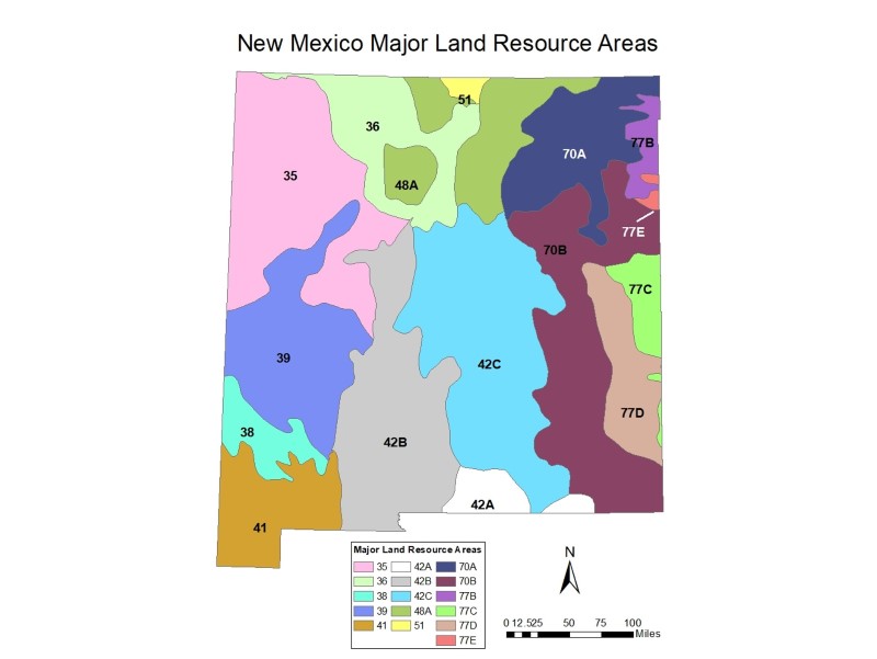
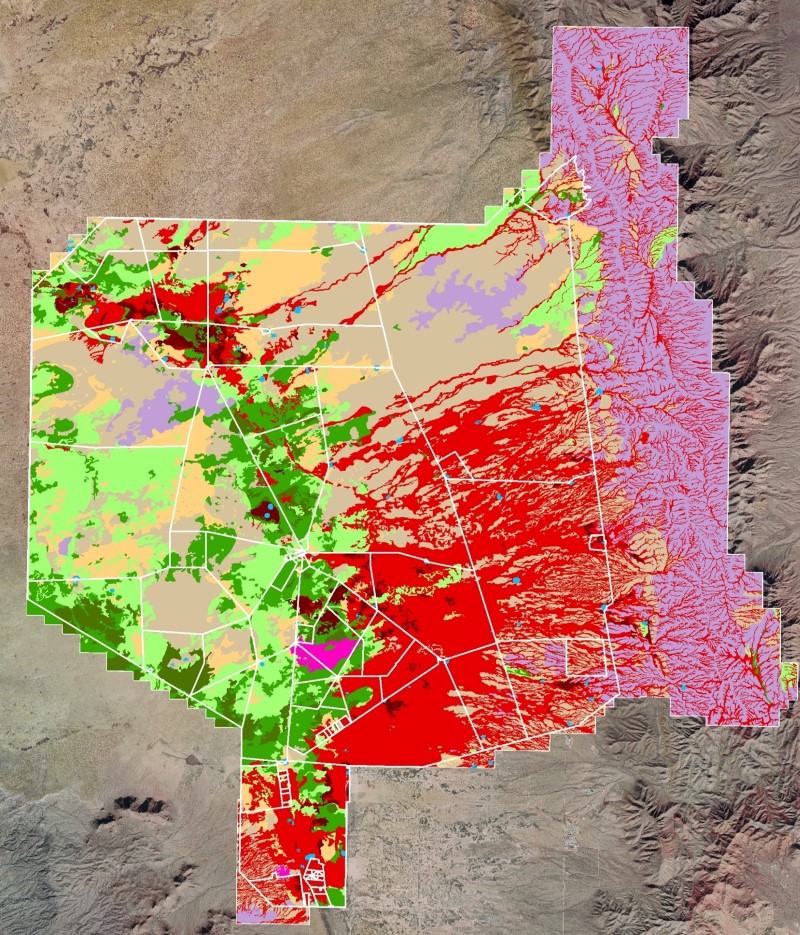
SSURGO soil maps within a given MLRA can be used to map ecological sites, which often occur in predictable patterns across the landscape. Illustrated here are the soil map units within MLRA 42B in New Mexico and Texas.
It is important to note that the accuracy of any given soil survey is related to (1) the scale at which the soil survey was conducted and (2) the age of the soil survey. Courser-scaled soil maps (1:24,000, 1:100,000) are less able to resolve individual soil components. Older soil surveys often did not have modern soil classifications and mapping procedures.
In the far right we have pulled out a small area within MLRA 42B to facilitate a discussion of soil map units and soil components.

Our focal area contains three soil map units. SSURGO polygons are identified by a soil map unit symbol. Each soil map unit symbol has its own unique name and represents one, or more than one, soil component (or soil series phase). It is helpful to think of a soil series as a “species,” and soil components as subspecies. The soil map unit symbols depicted here are RT (Rock outcrop-Torriorthents association), OP (Onite-Pajarito association) and SH (Simona-Harrisburg association). Focusing on SH, we can see that two major soil components comprise this soil map unit. Thus, 50% of the SH soil map unit is the Simona sandy loam, 1-5% soil component. The next major component of the SH soil map unit is the Harrisburg loamy sand, 1-5% component (25%). The remaining 25% of the soil map unit is comprised of six other types of soil (2 components and 4 series).

Mappers should review the properties of soil components in the mapping area. We can see here that the Simona sandy loam, 1-5%, soil phase is characterized by light brown sandy loam soils in the upper 8 inches. Then, from 8-12 inches soil color changes to pinkish white and finally a petrocalcic horizon is reached at 12 inches. In contrast, the top 8 inches of Harrisburg loamy sand, 1-5%, soil phase is coarser textured (loamy sand). This is followed by a texture and color change (light reddish brown sandy loam). Texture from 8-12 inches is similar for the two soil components, however, the petrocalcic horizon is considerably deeper in the Harrisburg loamy sand (24 inches). Understanding soil surface and subsurface color, as well as texture, assists with interpretation of imagery and verifying the ecological site. Color differences within imagery can be due to different soils, erosion of the same soil, and different plants.

Once we have identified the soil components present, the next step is to review ecological sites and their descriptions (ESDs). Each time you download a soil survey, the download comes with two folders (Spatial and Tabular). The tabular data contains an empty database and numerous tables. If you point the database to the folder where the tables are located, the database will import the data tables. This allows you to see each soil phase’s correlated ecological site. A given soil component can be correlated to only one ecological site. Each ecological site is typically associated with multiple soil components that are similar in their soil properties and potential plant communities.
Acquiring the ecological site correlated to each soil component allows the creation of a spatial data layer where each soil map unit is linked to its dominant ecological site(s).

Next, ecological site descriptions are reviewed, including their state and transition models (STMs). A clear understanding of each ESD, its soil properties, vegetation communities, states and transitions/pathways is crucial for interpreting imagery and delineating and attributing state polygons.

Overlaying the soil survey on DOQQs allows us to delineate state polygons within SSURGO soil map units. During the delineation process, soil map unit polygons are “cut” into smaller state polygons. The soil survey lines are preserved; polygons belonging to separate soil map units are never merged (even if they are the same ecological site and state). The state mapping technician uses the information gathered from ESDs and STMs when interpreting the imagery and determining where to divide ecological state polygons.

Where available, existing spatial data can assist with determining and attributing ecological site or state for a given polygon. At a minimum, the following spatial data layers should be available for any area in the United States: digital elevation model (DEM), MLRA, land ownership, and roads. The DEM is valuable for confirming elevation, and thus guiding the proper ecological site selection within a given MLRA. A spatial data layer for rainfall (e.g., PRISM = Parameter-elevation Regressions on Independent Slopes Model; PRISM Climate Group 2014, accessed 16 Feb 2023) can also be helpful.
Management boundaries are useful for distinguishing soil versus vegetation differences. Expert maps of vegetation, ecological sites or ecological states may already exist. These are most valuable for (a) unfamiliar and remote areas that are difficult or impossible to visit for field traverses and (b) confirming areas believed to be a specific ecological site or state. Downfalls of historic expert maps are predominantly related to the scale of the mapping effort (usually near 1:100,000); course scales lead to generalizations and corresponding incorrectly labeled ecological sites, states, or plant communities.
Geology and landform spatial data layers can be useful in determining ecological sites, especially where ecological sites are linked to parent materials derived from specific types of bedrock.

Any type of data that consists of a georeferenced point on the ground (UTM coordinates with a known coordinate system and zone) are valuable. Data may just contain coordinates and a photo. Sometimes these are accompanied by a plant community name. Also valuable are coordinates and a list of dominant species (with estimates of plant cover). The most valuable georeferenced ground data include: UTM coordinates, photo(s), soil profile characteristics, and detailed vegetation data (e.g., line-point intercept data providing canopy cover by species). Such data allow the technician to determine ecological site and state without local field work.

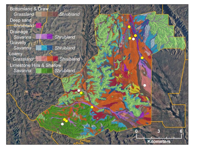
Often, georeferenced ground data do not exist. In that case, traverse data must be collected to verify states/ecological sites. Traverse data can be collected at low or medium intensity. In the image provided here, white points are low intensity traverse points, colored points are medium intensity. Each low intensity traverse point includes UTM coordinates, photos, an evaluation of Pedoderm and Pattern Classes, a list of the dominant 3 or 4 perennial plant species, and a designation of the ecological site and state. If a non-dominant focal species is present, it is also recorded (e.g., in MLRA 42B black grama is an important key species, honey mesquite and Lehmann lovegrass are important ‘invasive’ species). Medium intensity soil data includes a description of the key soil horizons at a site (A, B1, and diagnostic horizons), and an evaluation of Pedoderm and Pattern Classes. Medium intensity vegetation data include canopy cover classes for each perennial plant species, average plant height for dominant species, and percent of perennial grass cover growing within woody species (a measure related to the STM). A cover class is also assigned for the plot for all perennial grasses combined.

In the yellow box we can see white, low intensity traverse points, and multi-colored medium intensity points overlain on a DOQQ. Within the multi-colored medium intensity points, those of the same color represent the same ecological site and state. The two ground photos show two different traverse points. These traverse points have similar slopes, aspects and elevations. The field soil profile descriptions placed both points in the “Hills” ecological site, although the point in the upper left has lost almost all of its surface soil (A horizon). The point represented by the photo in the upper left would be considered in an altered grassland state with eroded areas to exposed bedrock. The point depicted in the lower right represents a mixed grass-shrub/succulent state with some shrub-dominated patches scattered throughout the landscape. Take time to contrast the percent of perennial grass cover between these two points, as well as the Pedoderm and Pattern Classes.
Traverse data are important data elements needed to attribute state polygons, but they also serve as data products that can be used down the road for management planning, monitoring and assessment extrapolation, etc.

In order to standardize the assignment of state codes to each polygon, each ecological site within an area of interest is grouped into a ‘Generalized Ecological Site’ class. This is typically done at the MLRA level. Members of generalized ecological site are structurally similar in their reference states and follow the same general STM. The generalized ecological site determines the possible ecological state codes. It is important to recognize and address potential weaknesses of ESDs and STMs during this process.
Once all the necessary data is gathered and overlain on DOQQs and generalized ecological state codes developed, polygons can be attributed with the ecological site and a three-digit state. The first number in the state code represents the dominant ecological state within the polygon of interest. The second digit represents the second dominant state, and the third is the third dominant state. Where only one or two states occur in a polygon, a zero follows the dominant state code(s). See Steele et al. 2012 for more information.


The final product is a state map that lists the ecological site name and the three-digit state code. State mapping is typically done at 1:4000 to 1:5000 m so this produces a fairly fine-resolution map. Recall that ecological state map polygons are child polygons of soil map unit polygons. Ecological state polygons attributed with the same ecological site and state code, but belonging to different soil map units are NOT merged. This allows ‘scaling up’ to create summaries at the soil map unit level, as well as analyses to be performed by soil map unit.

The state map provides spatially explicit delineation of ecological sites and states. State maps offer several advantages compared with ecological site maps offered through products such as the Web Soil Survey (https://websoilsurvey.nrcs.usda.gov). Spatial layers of ecological sites based strictly on soil map units provide the potential ecological sites based upon the dominant soil components in the soil map unit. The dominant ecological site is listed first; it is the ecological site correlated to the soil component comprising the most area within the soil map unit. Individual ecological sites typically are not spatially explicit, which can be problematic in soil map units with several components. In addition, the ecological sites that are linked to a soil map unit are only based on dominant soil components; soil inclusions are not represented. The spatial resolution of state mapping (1:13,000 – 1:16,000 ft) facilitates delineating ecological sites that occur at scales finer than that of the typical Order 3 soil survey (1:24,000 – 1:100,000 ft).

The state map also provides spatially explicit ecological states, which are linked to information of the STMs of ecological sites. The user can refer to ecological site descriptions and STMs to infer the potential of an area to respond to management and climate.

There are many potential uses for state maps. They are a useful tool for planning and prioritizing management efforts. State maps can be used to provide stratified randomization for monitoring efforts. Qualitative assessments can be extrapolated using state maps.

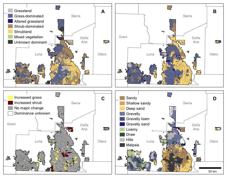
State maps can also be used to represent broad-scale patterns of state change. This example shows 1930s adjudication map polygons classified by A generalized ecological state based on 1930s data, B generalized ecological state based on 2005 data, C major state changes (a departure of 2 or more generalized states) between the 1930s and 2005, and D dominant ecological site. See Williamson, JC, et al., 2011.
State change detection can be performed by comparing historical vegetation maps against a modern state map for the same location. The state maps also lend themselves to tracking change into the future; the state map could be reattributed at some point in the future and analyzed to detect polygons that did and did not change, and whether the change involved an increase or decrease in shrubs, grass, etc.
The state map can be applied to determine where to focus limited management funds. Polygons in shrub-dominated and shrub-invaded grassland states, due to the presence of perennial grasses in those states, would have a greater potential to respond to shrub removal with an increase in grass cover than would shrubland states featuring few or no perennial grasses.

The state map can be used to allocate assessment locations using stratified random approaches within each of the dominant ecological sites and states can facilitate extrapolating point-based assessments to spatial units and entire landscapes.
Land managers and researchers can use state maps to determine the extent and location of focal states within a landscape.